4.2 Rheology

4.2 Rheology #

Lecture 4.2
Saskia Goes, s.goes@imperial.ac.uk

Learning Objectives #

Understand basic properties of elastic and viscous rheology and understand how the choice of rheology leads to different forms of the momentum conservation equation
Using tensor analysis to obtain relations between the main isotropic elastic parameters

Rheology #

deformation ($\boldsymbol{\varepsilon}$) = rheology $\cdot$ stress ($\boldsymbol{\sigma}$)

Rheology describes the material response to stress, depends on material, pressure, temperature, time, deformation history, and enviroment (volatiles, water).

experiments under simple stress conditions
elastic, viscous, brittle, plastic rheologies
strain evolution under constant stress, stress-strain rate diagrams
thermodynamics + experimental parameters
ab-initio calculations

Recap: Fluid - Solid #

What is a solid?

A solid acquires finite deformation under stress
stress $\boldsymbol{\sigma}$ ~ strain $\boldsymbol{\varepsilon}$

What is a fluid?

A material that flows in response to applied stress
stress $\boldsymbol{\sigma}$ ~ strain rate $\mathbf{D}$

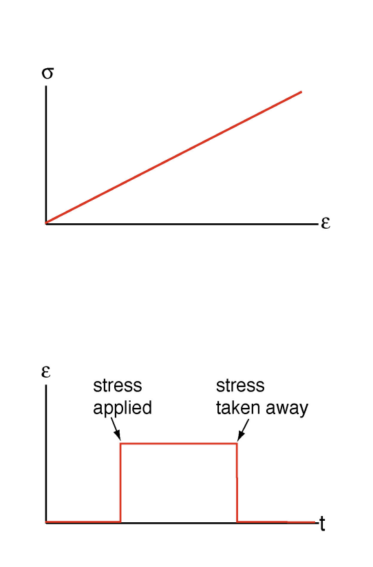
Elasticity #

linear response to load applied
instantaneous
completely recoverable
below threshold (yielding) stress
dominates behaviour of coldest part of tectonic plates on time scales of up to 100 m.y. => fault loading
on time scale of seismic waves, the whole Earth is elastic
$\sigma_{ij} = C_{ijkl} \epsilon_{kl}$ - Hooke’s law
$C_{ijkl}$ - rank 4 elasticity tensor, $3^4$ elements, up to 21 independent

Elasticity Tensor #

$C_{ijkl}$, $3^4 = 81$ elements (for $n = 3$)
symmetry of $\sigma_{ij}$ and $\varepsilon_{kl}$
$\Longrightarrow$ only 36 independent elements

\[P = \mathbf{\sigma :D} \approx \boldsymbol{\sigma} : D \boldsymbol{\varepsilon} / Dt = DU / Dt\]

conservation of elastic energy $U = \boldsymbol{\sigma} : \boldsymbol{\varepsilon} = \mathbf{C} : \boldsymbol{\varepsilon} : \boldsymbol{\varepsilon} \geq 0$
$\Longrightarrow C_{ijkl} = C_{klij} $
$\Longrightarrow$ only 21 independent elements - most general form of $\mathbf{C}$
other symmetries further reduce the number of independent elements

3 isotropic rank 4 tensors: $\delta_{ij}\delta_{kl}, \delta_{ik}\delta_{jl}, \delta_{il} \delta_{jk}$

For example, for isotropic media, only 2 independent elements ($\lambda, \mu$):

\[ \sigma_{ij} = \lambda \delta_{ij} \delta_{kl} \varepsilon_{kl} + \alpha \delta_{ik} \delta_{jl} \varepsilon_{kl} + \beta \delta_{il} + \delta_{jk} \varepsilon_{kl}\]

\[ = \lambda \delta_{ij} \varepsilon_{kk} + \alpha \varepsilon_{ij} + \beta \varepsilon_{ji} \]

\[ = \lambda \delta_{ij} \theta + (\alpha + \beta ) \varepsilon_{ij} \]

\[ \Longrightarrow \alpha_{ij} = \alpha \theta \delta_{ij} + 2 \mu \varepsilon_{ij} \]

Hooke’s Law for Isotropic Material #

2 independent coefficients

Lamé constants
$\mathbf{\lambda}$ and $\mathbf{\mu}$: $\sigma_{ij} = \lambda \varepsilon_{kk} \delta_{ij} + 2 \mu \varepsilon_{ij}$

Bulk and shear modulus
$K$ and $G$:
$ -p = K \theta $ - isotropic $-p = \sigma_{kk} /3 $
$ \sigma_{ij}^{'} = G \varepsilon_{ij}^{'} $ - deviatronic $ \theta = \varepsilon_{kk}$

Detemine relation to Lamé constants in Exercise 5

Young’s modulus and Poisson’s ratio
$E$ and $\nu$ : $E = \sigma_{11} / \varepsilon_{11}, \nu = -\varepsilon_{33} / \varepsilon_{11}$ (uniaxial stress)

Determine in optional Exercise 6

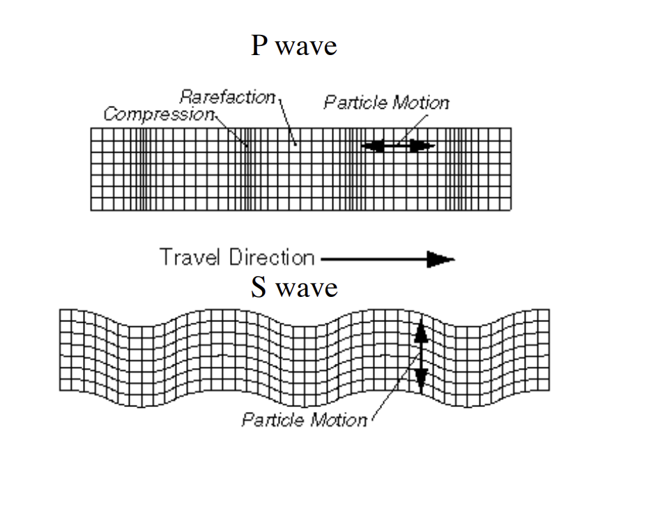
Wave Equation #

For infinitesimal deformation:
spatial coordinates ≈ material coordinates

$v_i$ (spatial) $\approx \partial u_i / \partial t$
$a_i$ (spatial) $\approx \partial v_i / \partial t = \partial^2 u_i / \partial t^2$

Equation of motion: $f_i + \partial \sigma_{ij} / \partial x_{j} = \rho \partial^2 u_i / \partial t^2$ (1)
Elastic rheology: $\sigma_{ij} = \lambda \varepsilon_{kk} \delta_{ij} + 2 \mu \varepsilon_{ij}$ (2)
Substitute (2) in (1) if (infinitesimal) deformation is consequence of force balance

\[ \partial \sigma_{ij} / \partial x_{j} = \lambda \partial \varepsilon_{kk} / \partial x_i + \mu \partial (\partial u_i / \partial x_j + \partial u_j / \partial x_i) / \partial x_j \]

\[ = \lambda \partial(\partial u_k / \partial x_k) / \partial x_i + \mu \partial^2 u_i / \partial^2 x_j + \mu \partial ( \partial u_j / \partial x_j) \partial x_i\]

\[ \mathbf{\nabla \cdot \boldsymbol{\sigma}} = (\lambda + \mu) \nabla (\nabla \cdot \mathbf{u}) + \mu \nabla^2 \mathbf{u}\]

Using: $\nabla^2 \mathbf{u} = \nabla (\nabla \cdot \mathbf{u}) - \nabla \times \nabla \times \mathbf{u}$

\[ \Longrightarrow \rho \partial^2 \mathbf{u} / \partial t^2 = \mathbf{f} + (\lambda + 2 \mu) \nabla (\nabla \cdot \mathbf{u}) - \mu \nabla \times \nabla \times \mathbf{u} \]

Where $(\lambda + 2 \mu) \nabla (\nabla \cdot \mathbf{u})$ represents compressional deformation,
and $\mu \nabla \times \nabla \times \mathbf{u}$ represents shear deformation

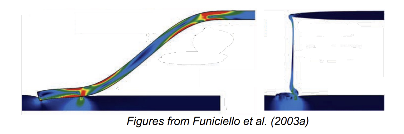
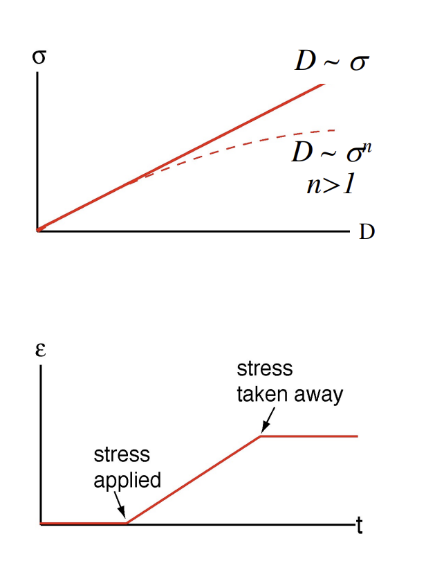
Viscous flow #

steady state flow at constant stress
permanent deformation
linear (Newtonian) or non-linear (e.g., Powerlaw) relation between strain rate and stress
isotropic stress does not cause flow
on timescales > years base tectonic plates and mantle deform predominantly viscously -> plate motions, postseismic deformation, but also glaciers, magmas

Hydrostatics #

Fluids can not support shear stresses
i.e. if in rest/rigid body motion: $\boldsymbol{\sigma} \cdot \mathbf{\hat{n}} = \lambda \mathbf{\hat{n}}$
and this normal stress is the same on any plane: $\mathbf{\sigma} = -p \mathbf{I}$

p is hydrostatic pressure In force balance:
$\nabla \cdot \boldsymbol{\sigma} + \mathbf{f} = 0$
$-\nabla p = - \mathbf{f}$

In gravity field $\frac{\partial p}{\partial z} = \rho g \Longrightarrow p_2 - p_1 = \rho g h$
where $h = z_2 - z_1$

Newtonian Fluids #

In general motion: $\boldsymbol{\sigma} = -p \mathbf{I} + \boldsymbol{\sigma}^{'}$

In Newtonian fluids, deviatoric stress varies linearly with strain rate, $\mathbf{D}$

\[ D_{ij} = ( \partial v_i / \partial x_j + \partial v_j / \partial x_i ) / 2 \]

For isotropic, Newtonian fluids, 2 material parameters:

Viscous stress tensor, $\sigma_{ij}^{'} = \zeta D_{kk} \delta_{ij} + 2 \eta D_{ij}$

where $\zeta$ is bulk viscosity and $\eta$ (shear) viscosity, $\Delta = D_{kk} = \nabla \cdot \mathbf{v}$

\[ \mathbf{\sigma} = ( -p + \varsigma \Delta) \mathbf{I} + 2 \eta \mathbf{D} \]

$p$ does not always mean normal stress: $\sigma_{kk} = -3p + (3 \zeta + 2 \eta) D_{kk}$

Consider a Newtonian shear flow with velocity field $v_1 ( x_2 ) , v_2 = v_3 = 0$

What is $\mathbf{D}$? What is $\mathbf{\sigma}$?

Exercise 7

Illustrates that $\eta$ represents resistance to shearing

Navier-Stokes for Incompressible Newtonian Flow #

For incompressible fluids $\Delta = 0$, so that:

\[\boldsymbol{\sigma} = -p \mathbf{I} + 2 \eta \mathbf{D}\]

Force balance: $$\nabla \cdot \boldsymbol{\sigma} + \mathbf{f} = \rho \frac{D\mathbf{v}}{Dt}$$

Show that:

\[ \frac{\partial \sigma_{ij}}{\partial x_j} = -\frac{\partial p}{\partial x_i} + \eta \frac{\partial^2 v_i}{\partial x_j \partial x_j} \]

Assuming constant $\eta$

\[ \sigma_{ij} = -p \delta_{ij} + \eta \left( \frac{\partial v_i}{\partial x_j} + \frac{\partial v_j}{\partial x_i} \right) \]

Hence,

\[ \frac{\partial \sigma_{ij}}{\partial x_i} = -\frac{\partial p}{\partial x_i} + \eta \left( \frac{\partial^2 v_i}{\partial x_j \partial x_j} + {\frac{\partial^2 v_j}{\partial x_i \partial x_i}} \right) \]

Note that: $${\frac{\partial^2 v_j}{\partial x_i \partial x_i}} = 0 \text{, as} \frac{\partial v_j}{\partial x_j} = \Delta = 0$$

Thus: $$ \frac{\partial \sigma_{ij}}{\partial x_i} = -\frac{\partial p}{\partial x_i}

\eta \left( \frac{\partial^2 v_i}{\partial x_j \partial x_j}\right)$$

In vector notation: $$ \nabla \cdot \boldsymbol{\sigma} = -\nabla p +\eta \nabla^2 \mathbf{v} $$

This makes the Navier Stokes equation of motion (Assuming constant $\eta$): $$ - \nabla p + \eta \nabla^2 \mathbf{v} + \mathbf{f} = \rho \left[ \frac{\partial \mathbf{v}}{\partial t} + \mathbf{v \cdot \nabla v} \right]$$

Together with continuity:

\[ \nabla \cdot \mathbf{v} = 0 \]

This makes a system of 4 equations with 4 unknowns ($p, v_x, v_y, v_z$)

Navier-Stokes for Compressible Newtonian Flow #

For compressible fluids $\Delta \neq 0$, so that:

\[\boldsymbol{\sigma} = (-p + \varsigma \Delta) \mathbf{I} + 2 \eta \mathbf{D}\]

\[\sigma_{ij} = -p \delta_{ij} + \zeta \frac{\partial v_k}{\partial x_k} \delta_{ij} + \eta \left( \frac{\partial v_i}{\partial x_j} + \frac{\partial v_j}{\partial x_i} \right)\]

Assuming constant $\eta, \zeta$

\[ \frac{\partial \sigma_{ij}}{\partial x_j} = -\frac{\partial p}{\partial x_i} + \zeta \frac{\partial^2 v_j}{\partial x_i \partial x_j} + \eta \left( \frac{\partial^2 v_i}{\partial x_j \partial x_j} + \frac{\partial^2 v_j}{\partial x_i \partial x_j} \right)\]

\[ \frac{\partial \sigma_{ij}}{\partial x_j} = -\frac{\partial p}{\partial x_i} + (\zeta + \eta) \frac{\partial}{\partial x_i} \frac{\partial v_j}{\partial x_j} + \eta \frac{\partial^2 v_i}{\partial x_j \partial x_j}\]

In vector notation: $$\nabla \cdot \boldsymbol{\sigma} = - \nabla p + (\zeta + \eta) \nabla (\nabla \cdot \mathbf{v} ) + \eta \nabla^" \mathbf{v} $$

Substituting this into the force balance gives the Navier Stokes equation of motion (Again assuming constant $\eta, \zeta$):

\[ - \nabla p + (\zeta + \eta) \nabla \Delta + \eta \nabla^2 \mathbf{v} + \mathbf{f} = \rho \left[ \frac{\partial v}{\partial t} + \nabla \mathbf{v \cdot v} \right] \]

Together with the conservation of mass for compressible material:

\[ \frac{D \rho}{D t} + \rho \nabla \cdot \mathbf{v} = 0 \]

and the energy equation for temperature $T$

plus an equation of state for $\rho (T,P)$

This yields 6 equations with 6 unknowns ($p, v_x, v_y, v_z, \rho, T$)

Recap #

Conservation equations
Energy equation
Rheology
Elasticity and Wave Equation
Newtonian Viscosity and Navier Stokes

More reading on the topics covered in this lecture can be found in, for example: Lai et al. Ch 4.14-4-16, 6.18, Ch 5.1-5.6, Ch 6.1-6.7; Reddy parts of Ch 5 & Ch 6

Practise #

For this part of the lecture, first try Exercise 5 and 7 in chapter4.ipynb

Then complete any remaining exercises in chapter4.ipynb:
Exercise 1, 2, 3, 4, 5, 7, 8
• Additional practise: in the text
• Advanced practise: Exercise 6